Processing of Raw Data Acquired from the APD

• The APD has an internal linear preamplifier, the output voltage is proportional to the x-ray intensity.  The linearity is checked before each series of measurements as very high x-ray intensity can cause saturation.
• The APD signal is directed into a digitizing oscilloscope.  At each x,y position, the oscilloscope averages the results of several sprays, and the data is then transferred to a PC for storage.  Note that all averaging is done in the oscilloscope, and only the final averaged results are stored on the PC. Therefore, we do not typically keep the single-shot results.
• The "raw" APD data looks like the following:
  


• If we expand the time axis of this plot, we can zoom in on the region of interest indicated by the box labeled "zoom region".  This looks like the following:
  
  


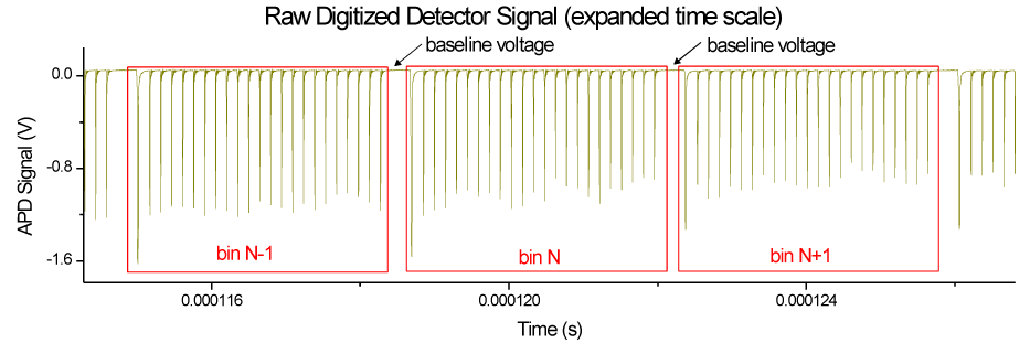
• Note that the APD response is a negative voltage signal, each pulse of the APD signal corresponds to a single x-ray pulse.  The APD pulses are ~10 ns wide (FWHM), therefore our digitizer must record a data point every 2 ns at the slowest in order to capture the shape of these pulses. Also note the repeating pattern of the APD pulses.  This is due to the fact that we are using a synchrotron source, the pulse pattern repeats every 3.6825 microseconds, which is the time of a single orbit around the synchrotron.  For this particular data set, there is a single large pulse followed by 22 smaller pulses and then a gap, all equally spaced around the synchrotron.  Note that this pulse pattern can vary depending on the operating mode of APS.  Each individual x-ray pulse does not contain enough photons for a statistically significant measurement of the x-ray absorption, therefore we combine the results from several consecutive x-ray pulses to get a statistically significant measurement.  This process is illustrated in the image above.  For each red box, all of the pulses inside that particular box are "binned" together by summing the integration of each individual peak. In effect, we are decreasing our time resolution to gain statistics.  Each of the time bins then contributes a single data point to the following plot:
  
  


• In the image above, each data point represents a single bin from the previous image.  In effect, we are taking our original raw data and discarding all the extraneous information, with a time resolution of 3.682 microseconds. In our group, we refer to each time step in the above plot as a "Snapshot", as if we had a camera with a shutter speed of 3.682 microseconds.  Each snapshot is numbered starting from 1, and we sometimes interchange snapshot number for the time axis. In the image above, the first 100 microseconds of data is acquired before the spray has intersected the x-ray beam.  We use this region of the data as our incident beam intensity, and we normalize the entire plot to the average in this region.  In this way, the measurement is self-normalizing, and any attenuation from the x-ray windows, fuel droplets on the windows, detector response, beam intensity, etc are all normalized for every individual measurement.  This normalization process results in the following plot:
  
  


• The image above shows the x-ray transmission, in which the data has been normalized to the baseline x-ray intensity.  A transmission of unity indicates the full x-ray beam hitting the detector, less than one indicates that the beam has been attenuated by the spray.  Because we use a monochromatic x-ray beam, there is a simple relationship between the transmission and the mass of fuel in the path of the beam.  This is shown in the following image:
  
  


• In this image, we have converted from transmission to mass.  This is measured as a function of time, in steps of 3.682 microseconds.  Data in this form is much more compact than the raw data, is easier to manipulate, and results in very little loss of information.